TF-IDF for tabular data featurization and classification
At Enigma, the daily work is driven by knowledge discovery across thousands of public datasets. These data sets come from a variety of sources and vary in areas such as data quality, completeness, and formatting conventions. Therefore, categorizing that data is a crucial step in the analysis process.
This post describes some work we’ve done at Enigma to classify tabular data using natural-language processing (NLP) techniques. A key feature of the data we’re working with is a high occurrence of placeholder values, which introduces some interesting differences compared to NLP for human-language data.
Data Types
Data in the wild has a range of difficulty of accurate identification. For example, emails have a strict format, so identifying a piece of data as an email is relatively straight-forward. A somewhat more complex data type is a phone number, which has a less uniform structure. On the far-end of the complexity scale there are more free-form data types such as organization names and street addresses.
Classification of data
Featurization of Cell Level Values
In our approach toward modeling data-type in a database column, we begin by featurizing the cell-level values. Many of these features are Boolean values that capture our human intuition about what’s important in determining the data type of a set of values. For example, in order to help classify emails we might generate features that say, “true or false - this value contains an @ symbol”, or “true or false - this value matches an email-format regex”. For phone numbers we might have features like “true or false - this value begins with a plus sign”, or “this value contains between 7 and 10 digits”. In practice we have dozens of such features that serve to describe a data point.
Database-Specific Complications
One complication of trying to classify database columns is the presence of placeholder values. For example, a column may be categorized as containing phone numbers, but contain a mix of authentic phone numbers and placeholders to signify missing values. If the placeholders are null or an empty string, then they’re straight-forward to identify and handle, but in practice different databases might choose different values, e.g. “—”, “.”, “NONE”, and etcetera. It’s not practical to keep a list of all possible placeholder values; nor would it be useful, since they can vary from system to system.
Useful natural-language processing (NLP) concepts for tabular data classification
Stop Words
The concept of placeholder values in database columns is conceptually similar to the concept of stop words in natural language processing (NLP). That is, words such as “the”, “of”, “a”, etcetera, that are common in documents of any topic and therefore don’t carry any semantic significance. A common practice in NLP is to identify a language / domain specific set of “stop words”, and remove them from the data before doing any additional analysis. In the database application, this would correspond to identifying common placeholder values and removing them before analyzing the column. In principle this is a theoretically justified, and practically useful, step to take, but the complications are choosing a threshold of occurrence frequency for defining a stop word, and in generating new stop word lists for each new database.
TF-IDF
A related analysis tool in NLP is term-frequency inverse-document-frequency (TF-IDF) which provides a concise way of representing the content of a document.
TF-IDF counts a term as being important to the identity of a document the more that term appears - this is the term-frequency component. However, the importance of a term is lessened according to the frequency that it occurs throughout the whole document set - this is the inverse-document frequency component, which effectively discounts terms that don’t have specificity. For example, if a document set comprises biographies of famous mathematicians, and cocktail recipes, the term “proof” may appear in all the documents, whereas a term like “calculus” would be more likely to appear in the mathematics articles. The TF-IDF approach can be viewed as a compromise between the extremes of giving all terms the same significance, and removing common terms entirely, as in the stop-words case (although in NLP work, stop-word removal and TF-IDF vectorization are both typically used). For classification work, using TF-IDF is appealing because it doesn’t necessarily require making a hard decision whether a term is in the stop-words list or not. Additionally, if there are class-specific placeholders, for example “1969-12-31” as a date-type placeholder, then the TF-IDF approach can make better use of that information than an approach that removed the class-specific placeholders as stop words.
More generally, the term and inverse-document frequencies can be thought of as local and global frequencies. Accordingly, there many plausible ways of defining them, and we’ll discuss a few below.
A TF-IDF Experiment for Database Columns
The considerations described above led us to experiment with applying TF-IDF to database columns. As mentioned above, this concisely representing a set of values, and has the advantage of automatically accounting for commonly occurring placeholder values without requiring generating a custom stop-words list.
TF-IDF was developed to analyze human language and there are a number of substantive differences with the applying it to a database. For one, the term frequency distribution tends to be much more bifurcated. That is, for many data types, a term is either unique, or nearly so (phone numbers, IP addresses, UUIDs, etc) or exceptionally common (placeholders). The other primary difference is that the percentage of terms in a document that are made up by placeholders can be much higher than the corresponding percentage of stop words in a natural-language document. It’s not unheard of for a database column to contain greater than 99% placeholder values - the natural language equivalent would be if a Wikipedia article about musical instruments said “the the the the… (thousands of times) … the bassoon clarinet drum”. In the case of classifying data type, even a few meaningful values in a column can be be distinctive enough to allow classification. As shown below, this suggests a sub-linear term-frequency function would be helpful.
A Working Example
To illustrate this concept further, I’ll generate a couple simulated data sets, and run through what the analysis looks like. A Jupyter notebook accompanies this post that includes all the details.
Simulated data
Simulated Classes
The classes I simulate are:
- phone number
- UUID
- float number
- binary number
For email, phone number, and UUID, I use the Faker Python library, which provides generators of synthetic data for a variety of data classes. For float numbers, I generated random values from a uniform distribution in the range -180 to 180. For the binary numbers, I generated a sequence of 0s and 1s, each with a probability of 1/2.
The email and UUID classes represent data types that are relatively easy to identify, and the phone number class a data type that’s less easy to identify. The float and binary number classes represent more generic data types.
Simulated Placeholders
As simulated placeholder values, I use “-”, ““, and”0“. The frequency of placeholder values in each column is 90%. Note that”0” is both a placeholder in some contexts, and a valid “binary number” in others.
Featurizers
The Boolean featurizers for this analysis comprise:
- an email regex
- a check for phone number format
- a check for UUID format
- a check for integer format
- a check for floating point numerical format
- a check that the length is exactly 1
The technical definitions for these are provided in the accompanying jupyter notebook.
As an example, the features generated for the input “-” are:
<div class="code-wrap"><code>{'email': False, 'uuid': False, 'phone_number': False, 'is_float': False, 'is_int': False, 'is_len1': True}</code></div>
``
and for “18005551212”:
<div class="code-wrap"><code>{'email': False, 'uuid': False, 'phone_number': True, 'is_float': True, 'is_int': True, 'is_len1': False}</code></div>
These sets of binary features are converted to “words”, by casting the Boolean values as 1s or 0s and then forming a string out of them. For example, the “words” defined by the features of “-” and “18005551212” shown above are 000001 and 001110, respectively. The database columns are then interpreted as “documents”, where the terms are these feature “words”.
Results
After organizing the data into documents as described above, we apply TF-IDF vectorization, using scikit-learn. The TF-IDF model uses a “smooth IDF” formulation which adds one to the document count of each term; that is, computes the inverse document frequency as log(N/(1+nt)), instead of the more literal definition of log(N/nt). In the preceding, N is the total number of documents and nt the number of documents in which a given term t occurs at least once. In practice the next step in a classification analysis would typically be to train a machine learning model (e.g., random forest, neural network) using the components of the TF-IDF vectors as input features. However, that’s an unnecessary step for the purposes of exploring the TF-IDF approach here. Instead, we apply the t-distributed stochastic neighbor embedding (T-SNE) algorithm to visualize the similarities between TF-IDF vectors, within and between data classes. The plots below are in t-SNE coordinates which have no inherent meaning - what’s important is the relative positioning between points, not the values of their coordinates.
Figure 1 shows the result of applying TF-IDF to the actual terms of the database columns. Not surprisingly, the bifurcated distribution of term frequency prevents the TF-IDF algorithm from making useful distinctions among data classes.
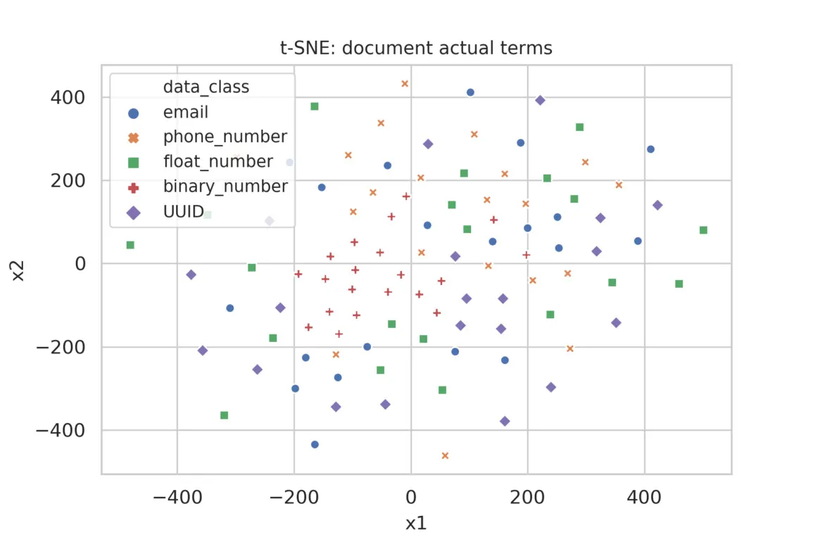
Figure 1
Figure 2 shows the result of applying TF-IDF to documents that are composed of the featurized words, as opposed to the actual terms. We see better separation of the data classes. Note that the clusters of phone number and binary number classes are near one another, indicating that there’s an inherent overlap between integers and phone numbers without string delimiters.
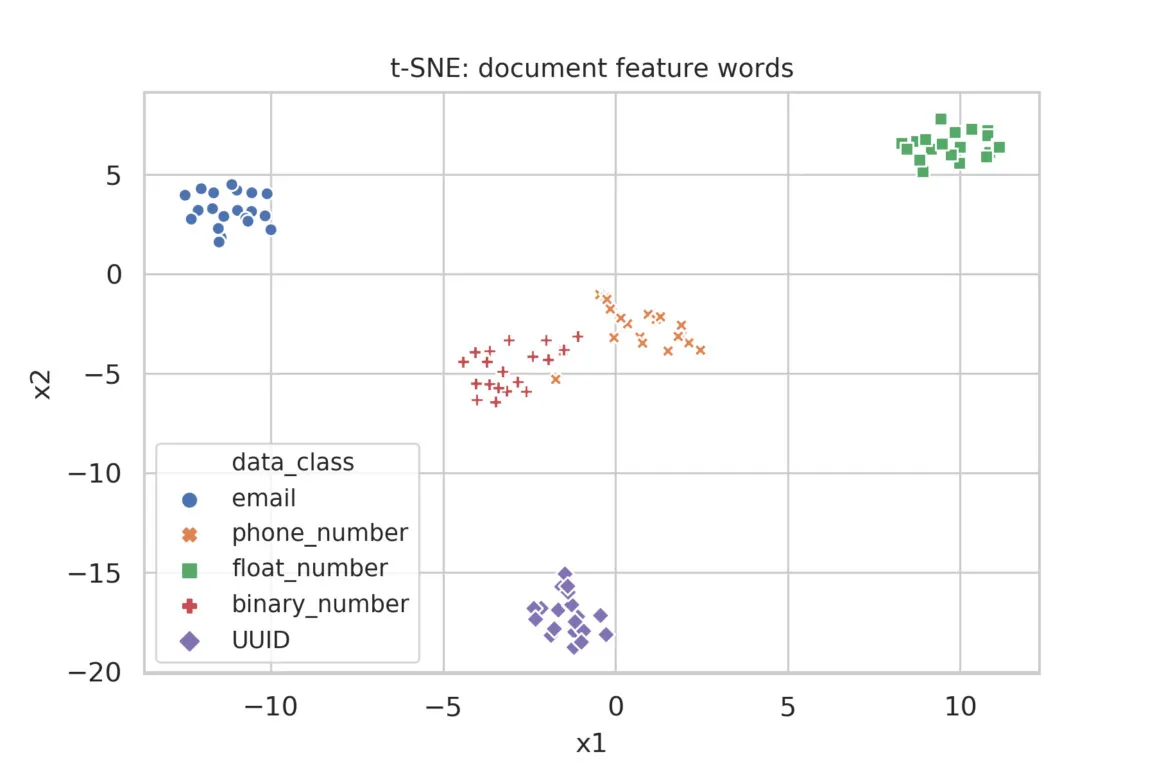
Figure 2
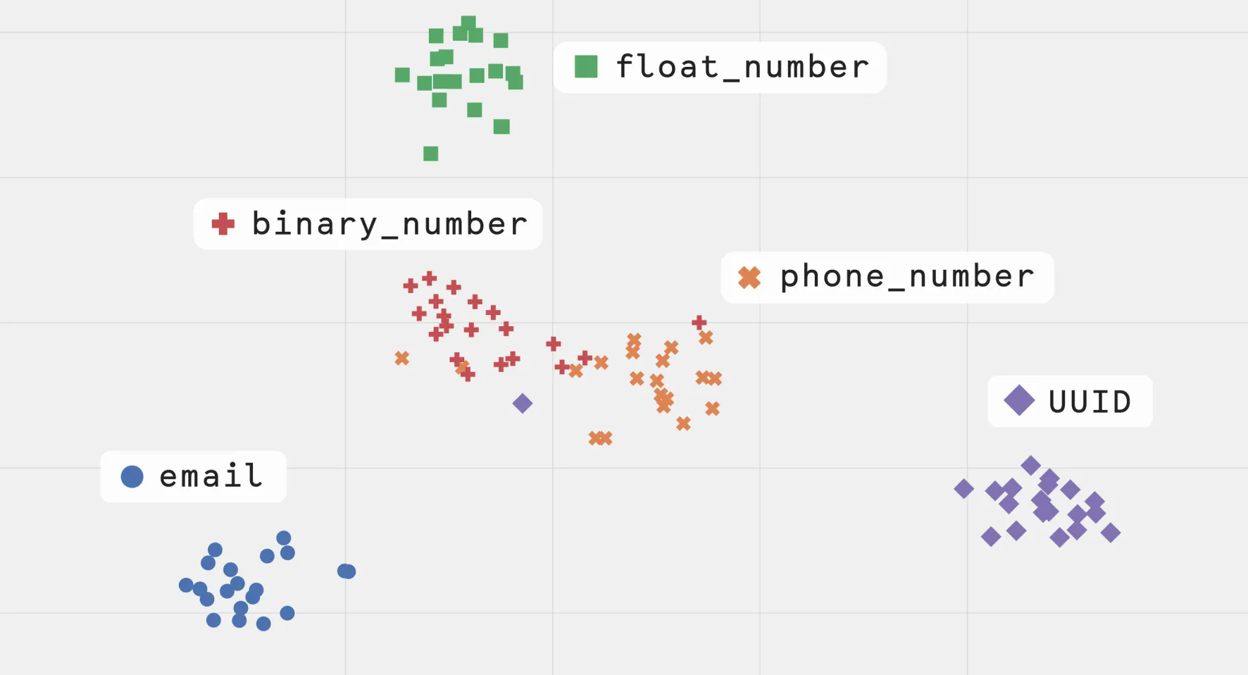
Finally, Figure 3 shows the result of the TF-IDF vectorization of documents of featurized words, with the modification of using a binary measure of local frequency, i.e. a word is counted with weight 1 no matter how many times it occurs in a document. In the database application, this is a way of applying a sub-linear term-frequency, thereby down-weighting frequent terms more strongly than might be necessary in a natural-language setting. We see the best separation of classes with this formulation.
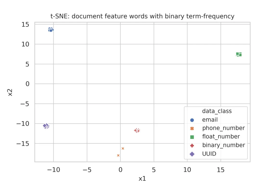
Figure 3
Conclusion
We have described a non-standard application of TF-IDF vectorization to a “non-natural” language, namely, database columns. We see that TF-IDF naturally accounts for placeholder values that can be common in a database environment. However, the distributional properties of terms within database columns are markedly different than those of natural-language. This means that performance is improved if a sub-linear term-frequency function is used. In particular, a binary term-frequency function is suitable for this example. Although this post describes the essential aspects of some experimentation we’ve done, in our day-to-day work at Enigma we extend the concepts presented here in several ways, including using a more complex feature set and applying supervised classification algorithms.